IoSR Blog : 2 June 2014
Computational Auditory Scene Analysis, part 3
Time–Frequency Masking: Reconstructing the Audio
In my previous blog posts (2013-12-16, 2013-10-23) I introduced some concepts related to computational auditory scene analysis (CASA) and especially time–frequency masking. Recall that time–frequency masking is a way of separating audio where we apply a gain to particular ranges of frequencies at particular points in time (or "time–frequency, T–F, units"). Hopefully we apply a negative gain to T–F units that are dominated by the sound that we don't want, and zero gain (no change) to the T–F units that are dominated by the sound that we want to extract. How we calculate those gains in practice is important, though a somewhat separate area of research. In my previous blog posts I showed how bad T–F masking can sound, but also suggested the ratio mask as one way to improve the sound [1]. In this post, I'll further explore how the gains could be set in order to obtain a result that sounds good (or at least better than it might have done).
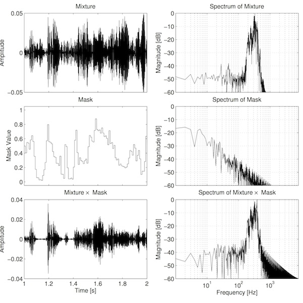
One way to think of T–F analysis is that we're passing the signal through many filters (something similar to one-third octave analysers) and separately recording the output of each of those filters. The masking process is simply applying a time-varying gain to the output of each of those filters, and then summing these results into a single signal. The time-varying gain is not usually calculated for every sample. In practice we need a number of samples over which to make measurements and calculate how to set the gain. We'll call this short time region, for making measurements, a frame. We calculate a gain for each frame, and then apply this gain to every sample in that frame. If we plot these gains over time then we'd see steps in the function at the boundaries between frames. See the example below.
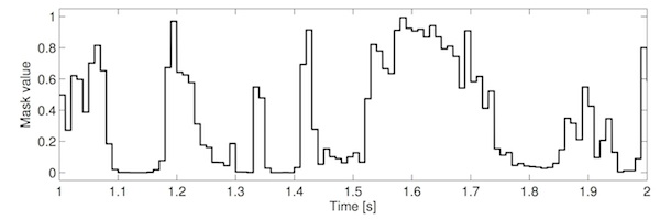
It seems intutitively reasonable that these step changes may contribute to the poor sound. Part of the reason for this relates to the concept of amplitude modulation. Simply put, amplitude modulation (AM) is when one signal is multiplied by another. In this case, the audio in each frequency channel is multiplied by the corresponding mask. The consequence of this amplitude modulation is that we generate new frequency components that were not present prior to modulation. Specifically we get two new "sidebands": one upper sideband consisting of frequencies determined by the sum of the mask and audio frequencies, and one lower sideband consisting of frequencies determined by the frequencies in the audio minus the frequencies in the mask. See the example below.
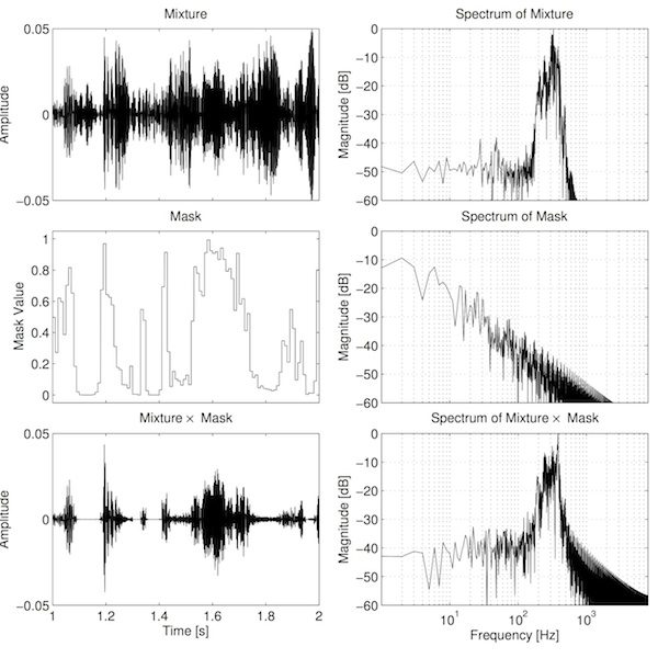
There are two important observations to make from this figure. Firstly, the spectrum of the mask is broad. This is primarily because of the step changes in the mask. The function is somewhat related to a square wave, and the sharp transitions create strong harmonics. Secondly, the new sidebands are clearly visible in the bottom-right plot, as there is additional energy at frequencies where there was previously less energy (e.g. above 1000 Hz). These sidebands are audible in the separated output as bubbly artefacts, similar to a bad audio codec.
What does this sound like in practice? Listen to the example below (I recommend using some good quality headphones or loudpeakers for these examples). Listen out for artefacts that sound bubbly or clicky. The bubbly artefacts are the extra frequencies introduced by the amplitude modulation. The clicks are due to larger step transitions in the mask.
Target (audio taken from the SiSEC 2010 database)
Interferer (audio taken from the SiSEC 2010 database)
Mixture
Ratio mask, stepped transitions
One solution to these problems, then, may be to smooth the mask by filtering it. This should remove or reduce some of the higher harmonics of the mask, thus narrowing the resulting sidebands. The process of framing the signal can be considered as a sampling problem. In these terms, the stepped mask seen above needs to be "reconstructed" to remove these steps. This process also happens at the output of a digital-to-analogue converter, where the audio is recovered from the stepped voltage by applying a so-called "reconstruction low-pass filter". The ideal filter for this purpose has an impulse response that follows the sinc function. The result is shown below.
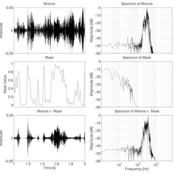
Again, two observations can be made from the plot. Firstly, the filter has been quite effective at removing the additional energy due to the higher harmonics present in the mask. Secondly, the filtering of the mask has introduced "ringing" artefacts in the mask (notice the ripples in the middle-left plot, especially around 1.8 s). This is an inherent problem with using a sinc filter. Sinc has a number of other problems: the impulse response needs to be very long in order to achieve a useful amount of filtering, and it introduces delay equal to half the impulse response length. In other words, the more filtering you want, the longer you have to wait for it! In fact, the ideal filter has an infinitely long impulse response! However, reasonable results can be obtained with a practical filter: listen to the example below. It should sound slightly less bubbly and much less clicky.
Ratio mask, sinc transitions
There are alternatives of course. In the next example I've used a Gaussian function, which seems to achieve a good balance of filtering whilst not introducing ringing, as shown in the graph below. You can listen to an example below too. It sounds pretty similar to the previous example.
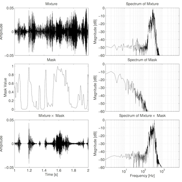
Ratio mask, Gaussian transitions
The ratio mask is relatively popular because it is "ideal", in that it maximises the amount of unwnated sound energy that is removed. But in the audio world, this doesn't necessarily mean that it sounds the best. This phenomenon, whereby what measures best is not necessarily what sounds the best, is seen time and again in audio. This was a principle consideration in the IoSR's recent Perceptually Optimised Sound Zones (POSZ) project (in collaboration with CVSSP and Bang & Olufsen). So it seems likely that we can find a mask that doesn't necessarily maximise the suppression of unwanted energy, but sounds better when we listen to it.
With this in mind, recent research at the IoSR has investigated changing the gain in such a way as to reduce the size of the step transitions between frames [2]. Recall that the ratio mask is calculated as the ratio of target power (in each T–F unit) to the sum of the target and interferer powers. The "sigmoid" mask is calculated by raising these signal powers to some numeric power. The mapping between ratio values and sigmoid values is shown below.
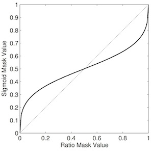
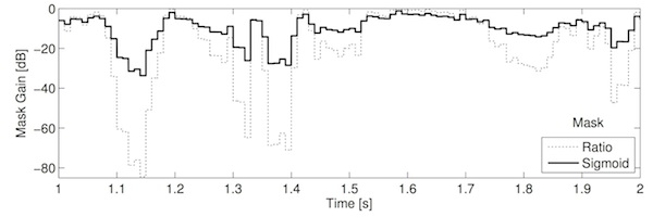
The reduced/compressed range occupied by the sigmoid mask is clear in the plot. This reduces the magnitude of the transitions between frames, thus reducing the magnitude of the high frequency components of the mask seen above. This results in less energetic sidebands and hence less audible artefacts. However, because it uniformally applies less gain to unwanted regions, it actually lets through more interference than the ratio mask. Toby's [2] paper explores this trade-off—between artefact reduction and interference suppression—in more detail (the value chosen here is the optimum value identified in his paper). See the plots and audio example below. You should hear slightly less clicky artefacts compared the ratio mask, but a slight "pumping" of the interfering sound.
Sigmoid mask, stepped transitions
Of course we can combine these ideas. Below is a combination of the sigmoid mask and Gaussian smoothing.
Sigmoid mask, Gaussian transitions
To conclude, we've seen how choosing the right gains makes a big difference to how good time–frequency masking can sound. We've seen a dramatic improvement in the sound quality compared to the binary mask, although we still have some way to go before time–frequency masking is good enough for high-quality audio systems. Somewhat counter-intuitively, choosing gains in order to maximise the amount of separation does not necessarily lead to an output that sounds best. This trade-off between good measurement and good sound is fundamental in psychoacoustics, and a guiding principle of much of the research undertaken at the IoSR.P.S. To save you scrolling up and down, here are all of the audio samples in one place…
Target (audio taken from the SiSEC 2010 database)
Interferer (audio taken from the SiSEC 2010 database)
Mixture
Ratio mask, stepped transitions
Ratio mask, sinc transitions
Ratio mask, Gaussian transitions
Sigmoid mask, stepped transitions
Sigmoid mask, Gaussian transitions
You can read more about these things in our researchers' new book chapter: 'On the ideal ratio mask as the goal of computational auditory scene analysis', in Blind Source Separation
.References
by Chris Hummersone